Global inversions, OH, and the stratospheric bias.

This is the finding that created Phase 2.

The finding [FR]

Eleven global inversions were evaluated against more than 50 AirCore balloon profiles collected at Sodankylä between 2013 and 2022 — profiles that measure methane directly, from the ground up to 25–30 km.

The pattern is systematic. Models overestimate methane in the stratosphere and underestimate it in the upper troposphere. Agreement is strongly altitude-dependent, and models represent polar vortex conditions poorly. Stratosphere–troposphere exchange rates and the stratospheric lifetime of methane are, plainly, not right. The single-flight comparison further down this page (under "Model and system development") illustrates the same kind of bias for one AirCore profile and one model resolution — the finding here is the same pattern confirmed across all eleven inversions and more than 50 profiles.

This is not an academic problem. Satellite instruments measure the total column — everything from the surface to space, stratosphere included. A stratospheric bias therefore leaks directly into the surface emissions an inversion infers. Independent confirmation comes from GOSAT: inversions using lower-tropospheric partial columns behave much like surface-data inversions, while total-column inversions produce substantially lower Northern Hemisphere emissions (Tsuruta et al., ACP, 2025).

Phase 2's WP2 exists to fix exactly this. See Phase 2.

What caused the methane surge? [TN2 §3.3.1]

Between 2019 and 2024 atmospheric methane grew unusually fast. Was that more emission, or less destruction? Methane is removed from the atmosphere mainly by the hydroxyl radical (OH), and if OH declined, concentrations would rise with no change in emissions at all.

SMART-CH4 ran TM5mp-4DVAR inversions over 2019–2024 at 3°×2° with 34 vertical levels, in seven configurations — surface data and satellite data, TROPOMI operational and WFMD, with and without OH optimisation — to separate the two explanations. This is one of the few places where a methane inversion system is asked to solve for the sink and the source at once.

Model and system development

TM5 was refined from 6×4×25 to 3×2×34 (lon × lat × layers) and coupled to the Community Inversion Framework in three modes — forward, 4D-Var and EnSRF — bringing a second major transport model into CIF alongside LMDz, CHIMERE, ICON-ART and FLEXPART.

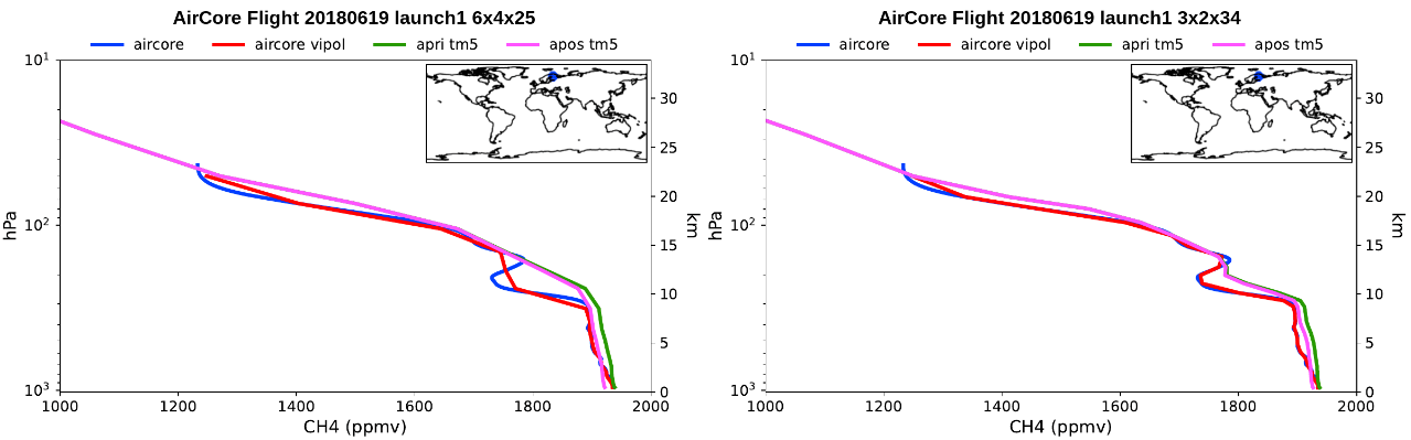
FMI ran CTE-CH4 inversions with TROPOMI/WFMD v2.0 and showed that inland-water priors materially change the split between biospheric and anthropogenic emissions, particularly north of 50°N.

Can land cover explain the wetland flux? [TN2 §3.4, FR]

If wetland emissions could be predicted from wetland maps, inventories would improve everywhere. Testing this against inversion output: roughly 80% of the variance in inverted biospheric fluxes is explained by a linear combination of wetland classes, with BAWLD classes plus GLWD peatland the best-performing combination (correlation 0.87). Marshes, fens and bogs carry the highest fluxes. Nonlinear fits overfit and are not recommended. The same method applied to separating agriculture from waste worked in the tropics (about half the variance in India, Bangladesh and Sri Lanka) but failed in Europe — population density, it turns out, is a poor proxy for where waste methane comes from.