Regional studies.
Four regional inversion efforts, spanning Europe, Romania, Scandinavia and the Tropics — each testing a different piece of the pipeline that turns satellite concentrations into emissions.
Europe: three TROPOMI products, three answers (LSCE / Science Partners) [TN2 §3.2.3, FR]
If two teams invert the same European emissions using two different TROPOMI products, do they get the same answer? Not yet.
Inversions with the SRON operational, IUP WFMD and BLENDED products give different posterior CH4 budgets at both pixel and country scale, and the EU27+UK total for 2019 remains inconsistent across products. OPER and BLENDED agree reasonably (BLENDED is a post-processed OPER, so this is expected); agreement with WFMD is poor. Temporal correlation is high across all three, and no product systematically converges toward a surface-based reference. BLENDED validates best against independent surface stations — but no product is uniformly superior.
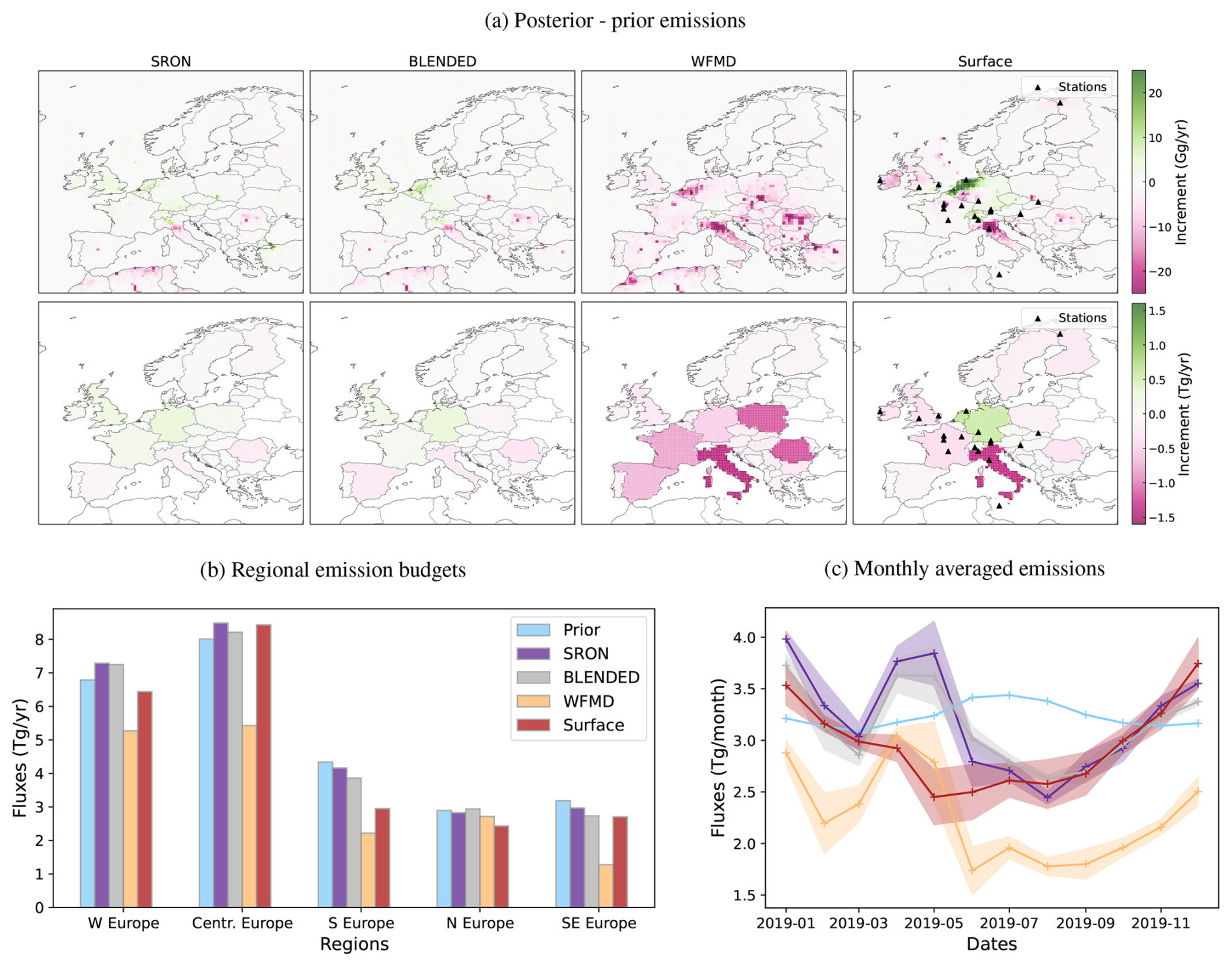
Machine-learning attribution (SHAP) identifies aerosols and surface albedo as the drivers of the inter-product differences. The inversion system's own sensitivity to background optimisation is a further, comparable source of spread. OSSEs are being used to disentangle observation density, error definition and vertical sensitivity (averaging kernels, prior profiles).
Published as Sicsik-Paré et al., ACP, 26(14), 10423–10454, 2026 (doi:10.5194/acp-26-10423-2026).
Why this matters: this is a warning about verification. If the choice of retrieval product moves a country's methane budget, then satellite-based national emissions reporting is not yet a solved problem — and saying so publicly is more useful than pretending otherwise.
Romania: watching an oil and gas sector clean up (Empa) [TN2 §3.2.1, FR]
Romania is one of the EU's largest oil and gas producers. The 2019 ROMEO campaign found something stark: 10% of production sites accounted for more than 70% of emissions, and total measured emissions exceeded what the entire Romanian oil and gas sector officially reports. A 2021 airborne campaign found super-emitter emissions had fallen by 20–60%.
Both estimates extrapolate from site-level measurements. SMART-CH4 tested them against the atmosphere: CIF–ICON-ART inversions at 3.3 km resolution, 90 vertical levels, an Ensemble Kalman Smoother with ~200 members, optimising emissions across ~10,000 regions, with priors built from CAMS-REG-GHG v4.2 plus site-specific ROMEO emission factors. Result: independent confirmation of a strong emission reduction between 2019 and 2021 (Kuhlmann et al., 2025) — with top-down totals still exceeding bottom-up reporting.
Scandinavia: wetlands, lakes and what the models miss (FMI) [TN2 §3.2.2]
Northern wetland emissions are heterogeneous in space, strongly driven by environment in time, and consequently among the most uncertain terms in the global budget. Earlier work found that inversions matched observations best when using the largest natural prior available — suggesting process-based models systematically underestimate methane from Finnish peatlands, or that something is missing altogether. Freshwaters are the leading candidate.
SMART-CH4 set up CIF–FLEXPART inversions at 0.1° over Finland and neighbouring countries, with priors assembled specifically for the problem: JSBACH-HIMMELI for wetlands (1.05 Tg/yr), GAINS+EDGAR v8 for anthropogenic sources (agriculture 0.30, waste 0.09, energy 0.04 Tg/yr), and lake emissions downscaled from Johnson et al. — retaining, importantly, the high per-area emission rates of small lakes (< 0.1 km²), which the coarse datasets tend to average away. AirCore profiles from Sodankylä and eddy-covariance flux towers provide independent validation.
The Tropics: where most of the methane is [TN2 §3.2.3, FR]
Africa, India/Southeast Asia and South America together account for roughly half of global methane emissions — and are the worst-observed. CIF–CHIMERE inversions were built for all three: South America at 0.2°, India/SEA at 0.35°, Africa at 0.3°.
For South America, six bottom-up inventories were first compared to establish how uncertain the starting point actually is:
| Sector | Mean (Tg/yr, 2019) | Spread across inventories |
|---|---|---|
| Wetlands | 67.5 | 42% |
| Agriculture & waste | 31.1 | 51% |
| Fossil fuels & industry | 8.0 | 77% |
| Biomass & biofuel burning | 3.6 | 36% |
Total: 108.5 Tg for 2019. The inversion assimilates 4.5 million TROPOMI soundings over the domain in that year, optimising fluxes weekly on a 250×275 grid, with background concentrations optimised alongside. Presented at EGU 2026 and the ICOS Science Conference 2026.
Read more:
- Sicsik-Paré et al., ACP, 2025; Kuhlmann et al., 2025; Mengistu et al. — Publications
- Global inversions and the stratospheric bias
- Phase 2, WP1 — merging point-source and regional scales